Decision Trees And Random Forests, All You Need To Know
We always hear about weak learners, but what is actually a weak learner? and how can we use it to make better classification models? In this article we will go through everything that you need to know about two of the most popular Machine Learning algorithms: Decision Trees and Random Forests, or also known as weak learners and how is it related to a Random Forest. After reading this post you should know the following:
- What is a Decision tree?
- Building the tree and measuring the impurity
- Gini impurity calculation
- When to stop splitting?
- Advantages and disadvantages of the Decision trees
- Python implementation of Decision tree
- What is Random Forest and why do we need it?
- Comparison between Decision tree and Random Forest
- Python implementation of Random Forest
- Resources & References
What is a Decision tree?
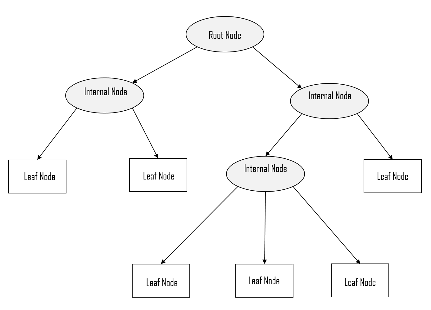
Decision trees is a supervised machine learning algorithm model that is used for both classification and regression tasks. Trees answer sequential “If-else conditional” questions in order to assign a class for the data. So, we begin from top to bottom by asking a question then classify the data based on the answers. We should first define some terminologies.
- The very top of the tree (first question) is called the “Root Node” or “The Root”
- The intermediate nodes or questions are called “Internal Nodes” or “Branches”
- The last nodes “the outputs” are called “Leaf Nodes” or just “Leaves”

An example for using the decision tree, notice we have:
- 4 Features : Condition (Old or New), Color, Model, Mileage and Brand
- 2 Labels / Output : Buy and Don’t buy

Building the Tree and measuring the impurity
To build a tree we will follow what we discussed in the terminology part. We will start with the root node. How to decide root node? Should I simply start with the condition because it comes first in the dataset?.
The answer to this comes from computing the impurity which then gives us a statistical measure such as:
- Information gain
- Gini index
- Gain Ratio
However numerically the methods are all quite similar, we will focus on Gini impurity, as it is the most popular and straightforward method
Gini impurity calculation
The metric measures the chances or likelihood of a randomly selected data point misclassified by a particular node. The Gini formula is straightforward, we calculate it for every feature and for every type of this feature then take the weighted average for each type. We will show an example.

Here P resembles the ratio of the specific j type of feature occurrence to the total number of occurrence of all types. Let’s explain more with a demonstrative example.

Let’s start with Credit Rating feature. It has 2 types (Fair and excellent) which will be our j as discussed above. We have only 2 labels (Yes and No).
This table means Credit Rating feature had 3 Fair entries that affect the output directly as Yes and 3 entries as No.
Therefore, to calculate the Credit Rating Gini index, we will first compute the type Fair.
Gini(Fair) = 1 – (3/(3+3))² – (3/(3+3))² = 0.5 (We divide here by 6 because we have 3 samples of Yes and 3 samples of No)
Gini(Excellent) = 1 – (2/(2+6))² – (6/(2+6))² = 0.375
Gini(Credit Rating) = Gini(Fair) * (6/6+8) + Gini(Excellent) * (8/6+8) = 0.429 (We divide here by 14 because we have 6 samples from Fair and 8 samples from Excellent)
After we compute the Gini index for all features, we take the lowest, as this resembles the lowest impurity which means it is the most important feature and we can take it as a root node.
The next step is to split the dataset by this chosen feature (root node). This means you will have 2 datasets, what we do is we take each dataset and compute the Gini index for all features for each one of them, and split again and again until we reach the leaf node.
If we have a huge number of features and we want to use all the features to build the tree, the tree will become too large. That may cause overfitting and long computation time.
When to stop splitting?
As we have seen previously, a problem usually has a large set of features, it results in large number of split, which in turn gives a huge tree. One way of solving this issue, is to set a minimum number of training inputs to use on each leaf. For example we can use a minimum of 10 samples to reach a decision(Yes or No), and ignore any leaf that takes less than 10 Samples. Another way is to set maximum depth of your model. Maximum depth refers to the the length of the longest path from a root to a leaf.
We can also improve the performance of a tree by pruning. It involves removing the branches that make use of features having low importance. This way, we reduce the complexity of tree and its overfitting.
Advantages and disadvantages of Decision trees
Advantages
- Simple to understand, interpret, visualize.
- Decision trees implicitly perform variable screening or feature selection.
- Can handle both numerical and categorical data. Can also handle multi-output problems.
- No feature scaling is required.
- The non-linearity relationship between the dependent and independent variables does not affect the performance of the decision tree algorithms.
- A decision tree algorithm can handle outliers.
Disadvantages
- Decision-tree learners can create over-complex trees that do not generalize the data well. This is called overfitting.
- Decision tree learners are weak learners and create biased trees if some classes dominate. Then, we might need to balance the dataset before using it to fit a model.
Python implementation of Decision Trees
First we import the needed libraries and load the dataset and reshape the data.
import numpy as np
import matplotlib.pyplot as plt
from keras.datasets import mnist
from sklearn.tree import DecisionTreeClassifier

(X_train, y_train), (X_test, y_test) = mnist.load_data()

X_train = X_train.reshape(X_train.shape[0],-1)
X_test = X_test.reshape(X_test.shape[0],-1)
Load the classifier and fit the training dataset
classifier = DecisionTreeClassifier(criterion='gini')
classifier.fit(X_train, y_train)
Predict on the test set
y_pred = classifier.predict(X_test)Also There are multiple ways to visualize what does the decision tree look like form inside and the decisions and conditions it made.
First way is by using tree.plot_tree
# Import Modules
from matplotlib import pyplot as plt
from sklearn import tree

names = np.arange(1,len(X_train[0])).astype(str)
classes = np.arange(0,10).astype(str)
# Create Figure with plot of Decision Tree
fig = plt.figure(figsize=(25,20))
_ = tree.plot_tree(classifier,
                   feature_names=names,
                   class_names=classes,
                   filled=True)
Since we are dealing with MNIST dataset that contains 28×28 images and then we flatten it to 784 features. It will be hard to see the tree but here what it looks like

The second way is by using graphviz, but it is too big to show it. So, we will show images on a different dataset that has less number of features.
from six import StringIO
from IPython.display import Image
from sklearn.tree import export_graphviz
import pydotplus

dot_data = StringIO()
export_graphviz(classifier, out_file=dot_data,
                filled=True, rounded=True,
                special_characters=True)

graph = pydotplus.graph_from_dot_data(dot_data.getvalue())
Image(graph.create_png())
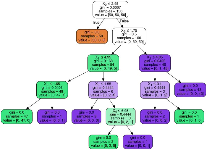
The following images are computed with the same codes above but on the Iris dataset that has only 4 features. In brief the iris dataset is about flowers and the features are the length and width of the petals and sepals ( petals and sepals are some parts of the flower )
This one is using graphviz

And this one is using tree.tree_plot which is the preferred method.

What is Random Forest and why do we need it?
We have discussed in the above section the problems of decision trees and that they are prone to overfitting. Here where Random Forest comes into play.
A Random Forest is simply a collection of decision trees whose results are aggregated into one final result. Their ability to limit overfitting without substantially increasing error due to bias is why they are such powerful models.
Random Forest reduces variance by training difference decision trees on different samples of data and thus, it is more robust than a single decision tree.
Step one of Random Forest : it takes a subset of the data, let’s say 2/3 of it and create a bootstrapped dataset. Bootstrap is nothing but dataset having the same size of input data, so if I have 100 entries (rows), Bootstrapped data will have 100 rows. The difference here is that we only take a random subset of it (2/3), but how will we get the same size as original?. Some of the data will be duplicated from the input data. The other 1/3 will be used to test on.
Step two of Random Forest : it randomly selects subset of features to be part of the root. (if you have 9 features, let’s say it randomly selects 3 features only that can be a root). Then calculates the Gini index that gives the best split of data or the maximum information. Then when it comes to the next node, the same is done.
In brief, if we have X training data points
- We can randomly split them into N datasets using bootstrapping
- Then form a tree from each dataset
- Then form a Random Forest from these N trees
- Then the final output will be decided using a major voting step on all the N trees outputs

Comparison between Decision trees and Random Forests

As we have seen previously, the first difference is that a decision tree depends on the output of the only branching graph created. While Random Forest takes a set of decision trees that work according to the output.
The only issue with Random Forest is that if you don’t have enough processing power or the dataset you’re working with is very large. They can take a long time to create. Also it is hard to be visualized.
Regarding Random Forest, It is complicated and we cant know which variable is used to split the data as it is more complicated because they are combinations of decision trees. While decision tree is simple and easy to interpret.
If we are going to compare accuracy, there is no doubt that Random Forest will perform better than one decision tree. Also, more trees will improve performance and make predictions more stable but will also slow down the computation speed.
Decision Trees And Random Forests Comparison
| Decision Tree | Random Forest | |
|---|---|---|
| Accuracy | The results are not accurate. | The results are accurate |
| Computation | Require low computation power | Require high computation power |
| Visualization | It is easy to visualize | This has complex visualization |
| Performance | Overfits the data | Does not overfit the data |
Python implementation of Random Forests
First we import the needed libraries and load the dataset and reshape the data.
import numpy as np
from keras.datasets import mnist
from sklearn.ensemble import RandomForestClassifier

(X_train, y_train), (X_test, y_test) = mnist.load_data()

X_train = X_train.reshape(X_train.shape[0],-1)
X_test = X_test.reshape(X_test.shape[0],-1)
Load the classifier and fit the training dataset
classifier = RandomForestClassifier(n_estimators = 100)
classifier.fit(X_train, y_train)
Predict on the test set
y_pred = classifier.predict(X_test)
Resources & References
- Full source code for Decision tree and Random forest implementation
- Explanation the measuring criteria using information gain
- Do we need normalization for the Decision trees?
- Step by step coding example


